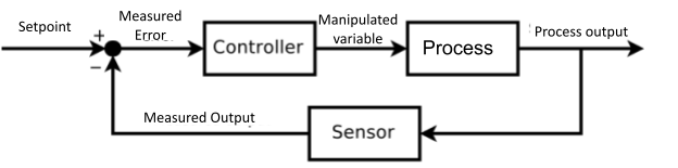
Process control is the science of maintaining key process parameters in manufacturing processes at their desired set points. Process controls can tune any controllable element of a process including heating and cooling, material flow rates, and pressure, and automatically make adjustments to system conditions to correct any measured deviations back to their expected values, also known as setpoints. The figure below shows an example of the logic used by a PID (proportional-integral-derivative) controller to make adjustments to a process. How this logic works is explained in detail in the section Feedback Control Modes.
Process control systems typically consist of a combination of measurement devices, final control elements, and computers. Basic process control elements include flow meters, pressure and temperature sensors, control valves, and other tools that measure process parameters or directly affect the process. Process control systems are programmable and can operate autonomously or respond to operator input. Higher-order control elements, such as input/output modules and supervisory computers, adjust the process parameters automatically when they see a process variable deviate from its set point.
Process controls are an added layer of safety to mitigate or prevent incidents such as overpressure, fires and explosions, and runaway reactions. They can also mitigate the effects of external disturbances such as temperature deviations. The level of automation process control allows for process optimization beyond what is possible with strictly manual control. This overview describes types of manufacturing processes and various types of control schemes, from controls of individual units to Distributed Control Systems (DCS) that control an entire plant.
Numerous forms of process control exist in the chemical industry. More simple processes may implement more basic forms of control such as feedback or PI control, while large, complex plants may integrate hundreds or thousands of control strategies into a distributed control system. Process control schemes exist for both economic optimization and as a safety measure, as controllers can be programmed to alert operators when process variables reach unsafe values. Controllers can be tuned for both continuous and batch processes, and different controllers are more useful in different process schemes.
Manufacturing Processes
Manufacturing processes can be categorized as a batch, continuous, or discrete. In a batch process, a fixed quantity of raw material is converted to a batch of the product, with definite beginning and endpoints. In a continuous process, on the other hand, continuous input flows are converted to outputs in a process that could operate 24 hours per day. In discrete processes, parts are assembled to produce individual items.
Batch manufacturing is typical for moderate quantities of products; foods and pharmaceuticals are typical industries that employ batch processing. Continuous manufacturing is designed for high-volume production; industrial chemicals and plastics typically employ continuous manufacturing. Discrete manufacturing is used in the production of items such as phones, cars, or other solid items. Each type of manufacturing requires a different form of process control.
Forms and Methods of Process Control
Two typical forms of process control systems are single input – single output (SISO) and multiple-input – multiple-output (MIMO). SISO is the simplest form of a control system: A measurement tool measures one process parameter, such as the system temperature, then converts it to an electrical signal. The actuator reads that signal to adjust a different process parameter, such as a coolant flow rate. Single-unit operations typically use SISO control schemes because the additional computing power required for a MIMO system is unnecessary. MIMO devices are more complex, as they are programmed to read numerous process parameters and adjust numerous operating parameters as needed. Distributed control systems (DCS), described in more detail below, consist of many MIMO devices spread across numerous units.
Control elements are typically described as feedback, feedforward, or a combination of both. Feedback control involves measuring the exit variable you wish to control, then manipulating input variables accordingly. In feedforward control, one measures a disturbance variable instead of the controlled variable to mitigate the effects of external factors, such as outdoor temperature, that may affect a process.
For example, consider the mixer shown below, in which two streams are combined in a ratio set by the process control system to create an exit stream with the desired composition:
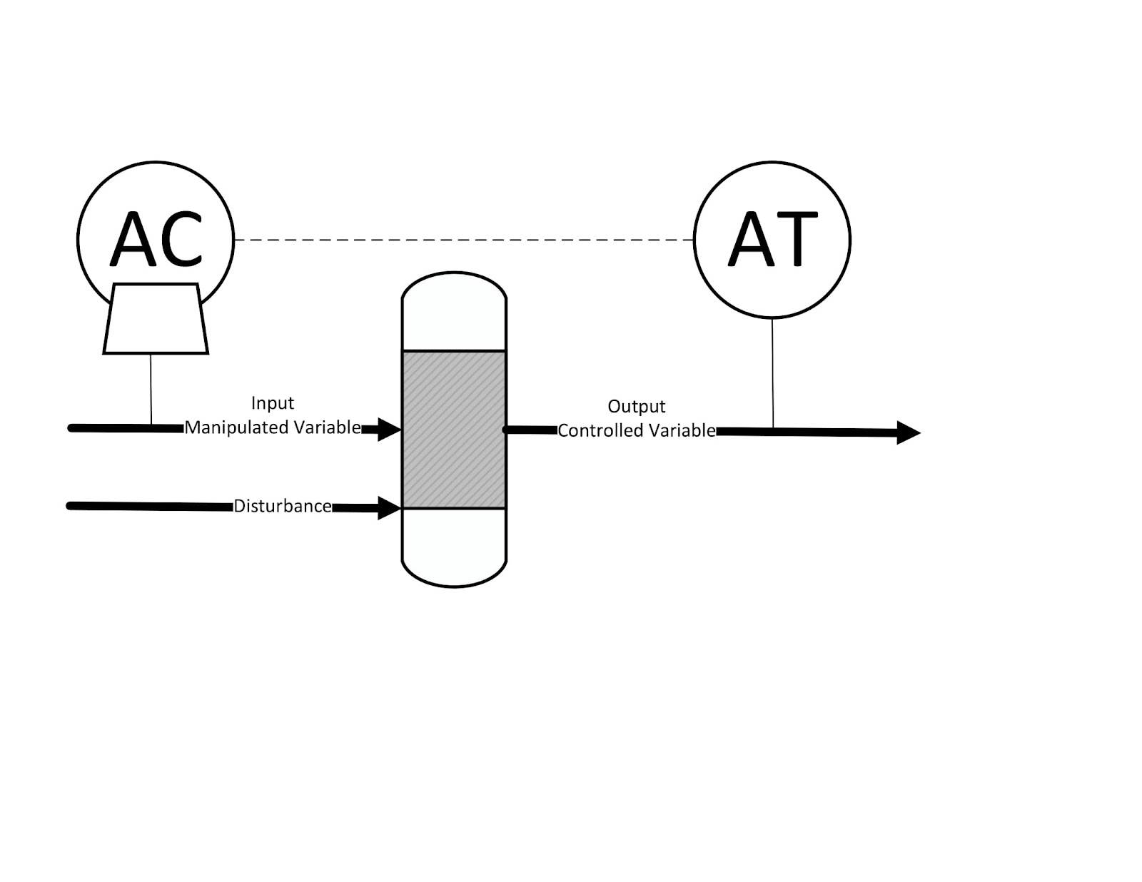
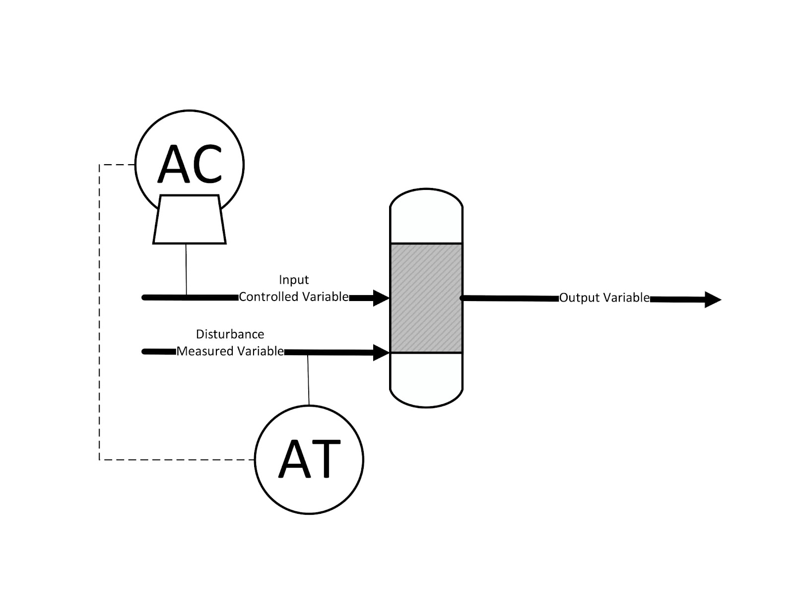
In feedback control, shown first, one would measure the composition of the output stream, convert that measurement to an electrical signal, then an actuator would read that signal and adjust the flow rate of one of the input streams as needed. A feedforward control loop, shown second, would measure the flow rate of the second input stream, then send an electrical signal to an actuator that would adjust the flow rate of the input stream to correct for any deviations and produce the desired output composition. A combination feedback-feedforward control loop consists of a device to measure the composition of an output stream and a ratio controller for two separate input flows that adjust both variables.
The main advantage of feedback control is that it is more practical and easier to implement than feedforward control. Disturbances are typically more difficult to measure than outputs, and feedforward control schemes only measure one disturbance. Feedforward control also requires a mathematical model of how each disturbance affects the output variable. Feedback control, on the other hand, measures the process output, which is affected by every process disturbance. The main advantage of feedforward control is that it measures disturbances before they can affect the output. In essence, feedforward control prevents deviations from the setpoint while feedback control responds to such deviations. Feedforward control is essential for time-sensitive operations where it is critical to prevent deviations from the setpoint before they occur.
Feedforward control is normally impractical to implement by itself, as it is impossible to measure every possible disturbance for a process, and disturbances can change over time. As such, hybrid feedback-feedforward control systems are typically used when a process requires feedforward control. The most critical disturbances are feedforward controlled, while the feedback control loop from the product stream accounts for other disturbances.
Alarms and Trips
Alarms and trips are basic safety features that make use of process controls. An alarm is an audio-visual cue to a control room operator that an abnormal deviation has occurred. Operators will then follow standard operating procedures (SOPs) to respond to the alarm. If the deviation exceeds a secondary limit or continues for an extended period of time, a safety trip will occur. Safety trips result in an automated response, such as pressure relief or emergency shutdown.
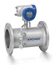
For example, if a set point for an exit flow rate is 300 L/min, an alarm may be configured to activate if a flowmeter reads above 330 or below 270 L/min. An alarm will notify the operators that a significant but not critical deviation has occurred and should be handled immediately. A safety trip sensor may activate if the reading exceeds 360 L/min or falls below 240 L/min. The emitted signal would automatically adjust a final control element such as a valve, coolant stream, or motor to correct the discrepancy. The figure below shows an ultrasonic flowmeter, a device that uses sonic waves to measure fluid flow rates. For more information about how this instrument works, see the velocity flowmeters article.
Feedback control modes
The three basic feedback control modes are proportional, integral, and derivative control. A feedback controller will incorporate one or more of those modes depending on the required degree of responsiveness to an error, where an error is defined as the difference between the measurement of the controlled variable and its setpoint. In proportional control, the controller output is proportional to the error, in integral control the controller output is proportional to the integral of the error over time, and in derivative control, the controller output is proportional to the derivative of the error with time. Feedback controllers may involve any of these control modes, but virtually all feedback controllers incorporate proportional control and the most common forms are Proportional Integral (PI) and Proportional Integral Derivative (PID) controllers, which involve combinations of the various modes of control.
Proportional Control
The controller output is a linear function of the error signal. The setpoint is pre-determined by the operator, then the sensor measures the output and compares it to the set point. The controller uses a gain constant that denotes the ratio of output to input variables. e.g. for each degree Celsius over a setpoint temperature, increase the coolant flow rate by 5 L/min. A proportional controller with a high gain will yield a fast response but can lead to instability because of the severity of the response to small errors. A low gain is more likely to maintain process stability but may not be sensitive enough to eliminate disturbances.
The most significant disadvantage of proportional-only control is there is no way to eliminate the error stemming from a setpoint change. Error stemming from a setpoint change is referred to as a steady-state error because the error is the result of calibration inaccuracies and not the result of a process disturbance. Proportional-only control is desirable for processes in which controlling steady-state error is less important. For example, a level controller for a tank may be more concerned with preventing overflow than maintaining the level at an exact set point.
Integral Control
The controller output is proportional to the integral of the error signal over a predetermined period of time. Essentially, the controller analyzes past errors to determine the output signal. Unlike proportional control, integral control takes into account the duration of the error and can eliminate steady-state error. Because integral control takes into account all errors over a period of time prior to producing a control signal, it is a much slower control method than proportional control. In addition, since integral control responds to the sum of all disturbances and setpoint changes, it runs the risk of overshooting the setpoint when producing its control signal. For these reasons, integral control is rarely used by itself; it is almost always used in conjunction with proportional control. Most industrial processes need to account for steady-state error; it is not typically tolerable for a process to produce a constant, unchecked error. As such, integral control is widely used in industrial control processes.
Derivative control
The controller output is proportional to the derivative of the error signal over a period of time. The purpose of derivative control is to predict future errors. Neither proportional nor integral control responds to immediate changes in a variable over a short period of time. Proportional control reacts to a deviation without regard to duration, while integral control only responds to changes over a long period of time. Derivative control responds to destabilizing disturbances and often offsets the destabilizing effects of integral control. Derivative control is never used by itself; it is always used in conjunction with proportional control and is often used in conjunction with integral control.
Distributed Control Systems
A distributed control system integrates many elements to control a whole section of the plant, composed of many processes. Before the distributed control system (DCS) was invented, every process within a plant was controlled by the single mainframe computer. This presented a safety concern because one technological failure could result in all processes losing control. A DCS is a hierarchical network of computerized process control elements. A typical DCS is both geographically and logically distributed, meaning that multiple control computers exist and are located throughout the plant.
The major priorities in setting up an automated Distributed Control System (DCS) are safety, production rate, product quality, cost, and stability. A DCS improves process safety by constantly monitoring process parameters such as temperature, pressure, or pH, to ensure they stay within their safe operating window. Failure to stay within these limits could lead to fire, explosion, or damage if left unchecked. Because a DCS can measure process parameters dozens of times per second, a DCS can alert operators and attempt to control problems much more quickly than a human can. A DCS can also constantly monitor product volume and adjust process parameters if production demands are not met or if the product is not sufficiently pure. A DCS can also be programmed to optimize process variables, such as minimizing energy usage and raw material demands. Furthermore, the automated nature of the DCS allows human operators to remotely operate a chemical process, which is particularly important for hazardous processes.
A DCS tends to be used on continuous, safety-critical processes because of the expense associated with numerous layers of control. A DCS will typically have four or five levels of control:
- Level 0 – Field instrumentation – sensors, transmitters, control valves
- Level 1 – Process connected control – Base level controllers, programmable logic controllers (PLC), process monitoring, such as analyzers.
- Level 2 – Supervisory Control – This includes the DCS system itself, and the main interface for operators.
- Level 3 – Advanced Control – Model predictive controls (MPC), non-linear controllers (NLC), detailed production scheduling, etc.
- Level 4 – Business and Information – usually a company’s business local area network. Some tools usually get developed here when analyzing historical process data. A lot of optimization and reliability analysis involves looking at historical data. Some companies also allow some plant unit overview displays to be seen at this level too. This allows personnel in remote locations, such as a company’s headquarters, to get a real-time view of the current performance.
Programmable Logic Controllers
Programmable logic controllers (PLC) differ from other controllers in that they primarily deal with digital (or binary) input rather than analog input. Because a PLC system is less expensive than a DCS, plants that can achieve satisfactory control with solely PLCs typically opt to do so, but they can also be used in conjunction with a DCS. While a PID controller will react to an analog electrical signal that can vary between 4 and 20 mA, a PLC will respond to numerous digital inputs. PLCs can handle thousands of digital inputs and outputs. These digital inputs may include whether a valve is open or shut or whether a motor is on or off. Particularly large-scale PLCs will double as analog controllers and provide PID control to processes as well. Much like a PID controller, a PLC will send an output signal to an actuator to adjust process variables depending on how it is programmed.
The process control strategies in previous sections are typically used in continuous processes. Batch processes are different than continuous processes because the process rarely reaches a steady state. Furthermore, since batch processes typically involve a much smaller quantity of product than continuous processes, equipment and control mechanisms are selected so that many types of batch processes can be performed using the same equipment. A programmable logic controller (PLC), is often used to account for variations in set points depending on the product being made.
Real-time Optimization
The process control elements mentioned so far adjust process parameters to minimize variation from a set point. Real-time optimization (RTO) is a strategy to adjust setpoints based on process data. RTO devices are higher-order than the DCS devices discussed above, and RTO takes place over a longer period of time than other process control strategies. While sensors collect data multiple times per second and actuators can adjust process variables multiple times per minute, set-point changes typically occur on the order of hours to days. RTO can be thought of as controlling a distributed control system, with the controlled variable being the DCS set points.
RTO is typically used to maximize the economic potential of a process. Every process variable has a maximum and minimum value; for example, pumps have a maximum throughput, and tanks have a maximum storage capacity. Variables are sorted into those that contribute to the process profit streams (end products), cost streams (raw materials), and the operating costs of the equipment. Operators then program the optimizer to maximize the profit stream while minimizing the cost streams. RTO is most effective when as many variables as possible are considered; large chemical plants take into account tens or even hundreds of thousands of input variables and optimize dozens of set points.
Because RTO implements so many variables, the models for each variable need to be relatively simple so the computer system can function quickly. RTO optimizers are typically linear, and the profit and cost streams are typically simple linear combinations of those models. More sophisticated models, such as quadratic or exponential, may reflect the actual process conditions more accurately, but the computing time required to optimize the setpoints would be too high to be effective.
Acknowledgements
- Krohne, Inc., Peabody, MA
References
- Cooper, D., & Houtz, A. (2015, April 9). The Feed Forward Controller. Retrieved September 18, 2017, from https://controlguru.com/the-feed-forward-controller/
- David R. Shay, personal communication, 2017
- Heavner, L. (2017, March). Control Engineering for Chemical Engineers. Chemical Engineering, 124(3), 42-50.
- Peter Martin, personal communication, 2017
- Seborg, D. E., Edgar, T. F., Mellinchamp, D. A., & Doyle, F. J., III. (2011). Process Dynamics and Control (3rd ed.). Hoboken, NJ: John Wiley & Sons, Inc.
- Towler, G., & Sinnott, R. (2013). Chemical Engineering Design (2nd ed.). Oxford: Butterworth Heinemann.
- Towler, G. (2017, February 8). Process Control Considerations in Process Design. Lecture presented at AICHE Webinar, from https://www.aiche.org/academy/webinars/process-control-considerations-process-design
Developers
- Joel Holland
- Austin Potter
- John Novak